In Part 1, we learned what makes graph databases different: data is stored as nodes (things) and relationships (connections), and those connections are first-class citizens in the database. We also wrote your first Cypher query to find patterns in banking data. Now it’s time to go deeper. In this article, lets learn how to create your own graph data, master essential Cypher clauses, and write the queries that make graphs truly powerful.

Table of contents

1. Graph Database Fundamentals: The Building Blocks
2. Setting Up Your Practice Environment
3. Creating Your Banking Graph
4. Essential Cypher Clauses
5. Wrap Up

Graph Database Fundamentals: The Building Blocks

Before we start creating data and writing queries, let’s establish a solid foundation by understanding the core concepts that make up Neo4j’s property graph model. These fundamentals will guide everything you do with graph databases.

The Property Graph Model

Neo4j uses a property graph database model. At its core, a graph data structure consists of nodes (discrete objects) that can be connected by relationships. Think of it like a network or mind map where circles represent things and arrows represent connections between those things. Here’s the simplest possible visualization.

(Node A) --[RELATIONSHIP]--> (Node B)

The Neo4j property graph model consists of five fundamental building blocks:

• Nodes - Represent entities or discrete objects in your domain
• Labels - Classify and group nodes into sets
• Relationships - Connect nodes and describe how they’re related
• Relationship Types - Classify relationships
• Properties - Store data as key-value pairs on both nodes and relationships

Let’s explore each of these in detail.

Nodes: The Things in Your Graph

Nodes are used to represent entities — the discrete objects in your domain. In our banking context, customers, products, accounts, and transactions would all be nodes.Key characteristics of nodes:

• A node can have zero or more labels
• A node can have zero or more properties
• Nodes can exist independently (a node doesn’t need relationships)

• The simplest possible graph is a single node with no relationships:

  (Customer)

Nodes represent the “nouns” of your domain — the people, places, things, or concepts that matter to your application.

Labels: Classifying Your Nodes

Labels shape your domain by grouping nodes into sets. All nodes with a certain label belong to the same set, which allows you to perform operations on specific types of nodes. Key characteristics of labels:

• A node can have zero to many labels
• Labels can be added or removed at runtime
• Labels are case-sensitive (:Person is different from :person)

Examples:

• All customer nodes could be labeled :Customer
• A person who is both a customer and an actor could have labels :Person:Customer:Actor
• You can use labels for temporary states: :Suspended for suspended accounts, :Active for active products
• In the example below, a single node has multiple labels to describe different dimensions: (tom:Person:Actor:Customer)
• This flexibility lets you query nodes from different perspectives. You might ask for “all Persons” in one query and “all Actors” in another, even if some nodes satisfy both criteria

Relationships: The Connections Between Things

A relationship describes a connection between a source node and a target node. This is where graphs truly differ from relational databases—relationships are not inferred or calculated; they’re stored directly as first-class data structures.Key characteristics of relationships:

• Connects exactly one source node to one target node
• Always has a direction (though you can ignore direction in queries when appropriate)
• Must have exactly one relationship type
• Can have properties (key-value pairs)

• A node can have a relationship to itself Example relationship:

  (alice:Customer)-[:USES {since: date(‘2020-01-15’), status: ‘active’}]->(savings:Product)

This shows:

• Source node: alice (a Customer)
• Relationship type: USES
• Direction: From alice to savings (indicated by ->)
• Properties: since and status stored on the relationship itself
• Target node: savings (a Product)
• Relationships always have a direction, but you can traverse them in either direction or ignore direction entirely when querying. The direction is part of the data model and can carry semantic meaning—”Alice USES Product” is different from “Product USED_BY Alice,” even though they describe the same connection from different perspectives.

• Important: A node can have a relationship to itself. For example, if Tom Hanks knows himself:

  (tom:Person)-[:KNOWS]->(tom)

Relationship Types: Classifying Connections

Just as labels classify nodes, relationship types classify relationships. Every relationship must have exactly one type. Key characteristics:

• A relationship has exactly one type (unlike labels, you can’t have multiple)
• Types define the semantic meaning of the connection
• Types are case-sensitive
• Common relationship types in banking:
  • :USES - Customer uses Product
  • :OWNS - Customer owns Account
  • :ISSUED_BY - Card issued by Bank
  • :TRANSFERS_TO - Account transfers to Account
• The relationship type tells you how two nodes are connected. This is crucial for traversals—when you follow relationships, you often want to follow only specific types. You might want to find “all products a customer USES” without including “all accounts they OWN.”

Properties: Storing Data

Properties are key-value pairs that store data on both nodes and relationships. They’re where you put the actual information about your entities and connections. Key characteristics:

• Properties are stored as key-value pairs
• Both nodes and relationships can have properties
• Values can be primitives (numbers, strings, booleans) or homogeneous arrays
• Properties are case-sensitive
• Naming convention: Use camelCase for properties (firstName rather than first_name)
• Supported data types:

Numbers:

CREATE (:Example {count: 42, price: 19.99})

Strings and booleans:

CREATE (:Example {name: 'Alice', active: true})

Dates and temporal types:

CREATE (:Customer {since: date('2020-01-15'), lastLogin: datetime()})

Arrays (homogeneous lists):

CREATE (:Example {
  tags: ['premium', 'verified'],
  scores: [95, 87, 92],
  active: [true, false, true]
})

Important: Properties are only stored when they have values. There’s no concept of null values being stored—if a property isn’t set, it simply doesn’t exist on that node or relationship.

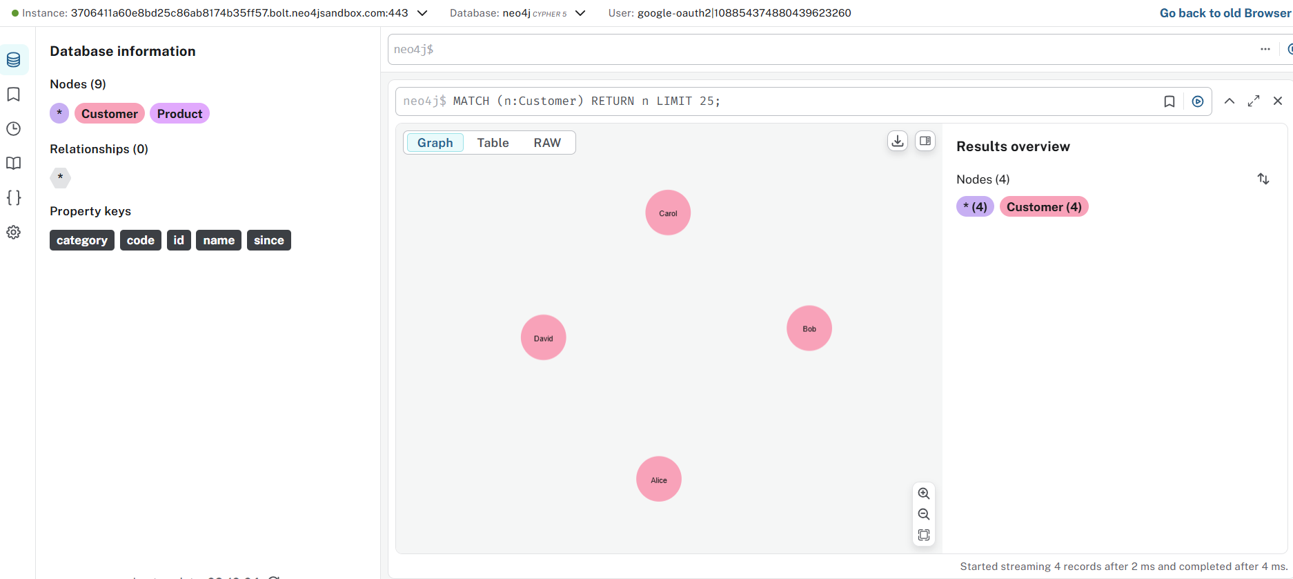
Setting Up Your Practice Environment

Neo4j Sandbox runs entirely in your browser—no installation required. Visit sandbox.neo4j.com, create a free account, and launch a blank sandbox. Within seconds, you’ll have a working Neo4j instance with the Browser interface ready to go. This is perfect if you want to start immediately without worrying about setup. If you’re using a sandbox that has sample data, or if you want to start fresh at any point, you can clear everything with:

MATCH (n) DETACH DELETE n

This finds all nodes (MATCH (n)), detaches them from their relationships, and deletes everything. This was very useful for the exercise below .

Creating Your Banking Graph

In Part 1, you queried existing data. Now you’ll learn how to create it yourself. Neo4j uses the CREATE clause to add nodes and relationships to your graph.

Creating Nodes

Let’s start by creating some customers. Each customer is a node with properties that describe them:

CREATE (alice:Customer {id: 'C001', name: 'Alice', since: date('2020-01-15')})

Let’s break down what’s happening here:

• CREATE tells Neo4j we’re adding something new
• (alice:Customer …) creates a node. The word before the colon (alice) is a variable we can use in this query, and the word after (:Customer) is a label that categorizes this node
• {id: ‘C001’, name: ‘Alice’, since: date(‘2020-01-15’)} are properties—key-value pairs that store information about this customer
• The date() function creates a proper date object rather than just text

Run that query, then create a few more customers:

CREATE (bob:Customer {id: 'C002', name: 'Bob', since: date('2021-03-20')})
CREATE (carol:Customer {id: 'C003', name: 'Carol', since: date('2019-07-10')})
CREATE (david:Customer {id: 'C004', name: 'David', since: date('2022-06-05')})

Each CREATE statement adds one node to your graph. You should see a confirmation message after each one: “Added 1 node.”

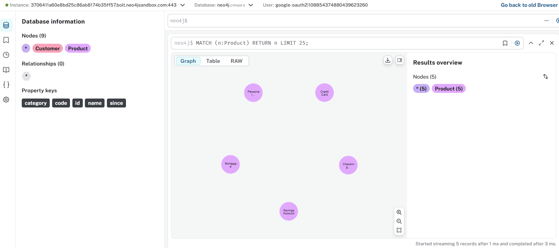
Creating Products

Now let’s add the banking products these customers might use:

CREATE (savings:Product {code: 'SAV-001', name: 'Savings Account', category: 'Deposit'})
CREATE (checking:Product {code: 'CHK-001', name: 'Checking Account', category: 'Deposit'})
CREATE (credit:Product {code: 'CRD-001', name: 'Credit Card', category: 'Credit'})
CREATE (loan:Product {code: 'LON-001', name: 'Personal Loan', category: 'Credit'})
CREATE (mortgage:Product {code: 'MTG-001', name: 'Mortgage', category: 'Credit'})

Notice we’re using different properties here (code, name, category) because products need different information than customers. This flexibility is one of the strengths of graph databases—different node types can have completely different properties.

Creating Relationships

Now comes the interesting part: connecting customers to products. This is where graphs really shine. We need to find the nodes we want to connect, then create a relationship between them:

MATCH (alice:Customer {id: 'C001'})
MATCH (savings:Product {code: 'SAV-001'})
CREATE (alice)-[:USES {since: date('2020-01-15'), status: 'active'}]->(savings)

Let’s understand this step by step:

• The first MATCH finds Alice (the customer we created earlier)
• The second MATCH finds the Savings Account product
• CREATE (alice)-[:USES …]-> (savings) creates a relationship from Alice to the Savings Account
• The relationship type is USES (inside the square brackets)
• The direction matters: the arrow -> points from customer to product, meaning “Alice uses Savings Account”
• Relationships can have properties too: we’re storing when the relationship started and its current status

Add several more relationships to build out our dataset:

MATCH (alice:Customer {id: 'C001'})
MATCH (credit:Product {code: 'CRD-001'})
CREATE (alice)-[:USES {since: date('2020-06-10'), status: 'active'}]->(credit)

MATCH (bob:Customer {id: 'C002'})
MATCH (checking:Product {code: 'CHK-001'})
CREATE (bob)-[:USES {since: date('2021-03-20'), status: 'active'}]->(checking)

MATCH (bob:Customer {id: 'C002'})
MATCH (credit:Product {code: 'CRD-001'})
CREATE (bob)-[:USES {since: date('2021-08-15'), status: 'active'}]->(credit)

MATCH (bob:Customer {id: 'C002'})
MATCH (loan:Product {code: 'LON-001'})
CREATE (bob)-[:USES {since: date('2023-01-10'), status: 'active'}]->(loan)

MATCH (carol:Customer {id: 'C003'})
MATCH (savings:Product {code: 'SAV-001'})
CREATE (carol)-[:USES {since: date('2019-07-10'), status: 'active'}]->(savings)

MATCH (carol:Customer {id: 'C003'})
MATCH (checking:Product {code: 'CHK-001'})
CREATE (carol)-[:USES {since: date('2019-07-10'), status: 'active'}]->(checking)

MATCH (carol:Customer {id: 'C003'})
MATCH (mortgage:Product {code: 'MTG-001'})
CREATE (carol)-[:USES {since: date('2020-11-20'), status: 'active'}]->(mortgage)

MATCH (david:Customer {id: 'C004'})
MATCH (credit:Product {code: 'CRD-001'})
CREATE (david)-[:USES {since: date('2022-06-05'), status: 'active'}]->(credit)

MATCH (david:Customer {id: 'C004'})
MATCH (loan:Product {code: 'LON-001'})
CREATE (david)-[:USES {since: date('2023-09-12'), status: 'active'}]->(loan)

After running all these queries, we’ve built a small but complete banking graph. We have customers, products, and the relationships between them—including metadata about when each relationship started and whether it’s currently active.

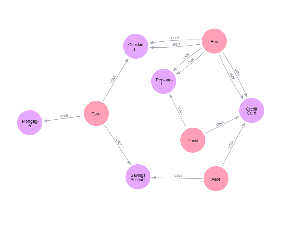
Verify Your Graph

Let’s make sure everything is there:

MATCH (c:Customer)-[u:USES]->(p:Product)
RETURN c.name, p.name, u.since
ORDER BY c.name, u.since

You should see all your customers, the products they use, and when they started using them. This is the graph you’ll query throughout the rest of this article

From Relational to Graph: A Mental Model Shift

If you’re coming from a relational database background, you might be wondering how the graph model you just created compares to what you’re used to. Let’s make that connection explicit. In relational databases, you would model our banking scenario with separate tables for Customers and Products, connected through a JOIN table (often called Customer_Product or similar). That JOIN table would contain foreign keys pointing to both tables, plus any relationship metadata like since and status. In Neo4j, we’ve eliminated that intermediate JOIN table entirely. The relationship itself is the connection, and it carries the metadata directly. No foreign keys, no JOIN table, no extra lookup step.

What you gain:

• Direct connections: Relationships physically point from one node to another
• Constant-time traversals: Following a relationship doesn’t require index lookups or table scans
• Clearer model: What you sketch on the whiteboard is what you store in the database

This is what we mean by “index-free adjacency”—each node directly references its relationships, making traversals extremely fast regardless of database size

Essential Cypher Clauses

You now have data in your graph. To ask useful questions of it, we need to master the core Cypher clauses that filter, shape, and aggregate your results. These clauses are the building blocks of every query you’ll write.

WHERE: Filtering Your Results

The WHERE clause lets you filter nodes and relationships based on their properties. In Part 1, you saw simple property matching like {name: ‘Alice’} directly in the MATCH pattern. WHERE is more flexible and handles complex conditions. Find all customers using Credit products:

MATCH (c:Customer)-[:USES]->(p:Product)
WHERE p.category = 'Credit'
RETURN c.name, p.name

The WHERE clause filters after the pattern is matched. Only relationships where the product category equals ‘Credit’ will appear in results. You can combine multiple conditions:

MATCH (c:Customer)-[:USES]->(p:Product)
WHERE p.category = 'Credit' AND c.since > date('2021-01-01')
RETURN c.name, p.name, c.since

This finds customers who joined after January 2021 and use Credit products. Use OR for alternatives:

MATCH (c:Customer)-[:USES]->(p:Product)
WHERE p.category = 'Credit' OR p.category = 'Deposit'
RETURN c.name, p.name, p.category

You can also filter on relationship properties:

MATCH (c:Customer)-[u:USES]->(p:Product)
WHERE u.status = 'active' AND u.since > date('2022-01-01')
RETURN c.name, p.name, u.since

This finds only active relationships that started after 2022. Notice we gave the relationship a variable (u) so we can reference its properties.

Comparison operators work as you’d expect:

MATCH (c:Customer)-[u:USES]->(p:Product)
WHERE u.since < date('2021-01-01')
RETURN c.name, p.name, u.since
ORDER BY u.since

The <> operator means “not equal”:

MATCH (c:Customer)-[:USES]->(p:Product)
WHERE p.category <> 'Deposit'
RETURN c.name, p.name

ORDER BY and LIMIT: Controlling Output

ORDER BY sorts your results, and LIMIT restricts how many rows you get back. These are essential when exploring data or building user-facing features. Sort customers alphabetically:

MATCH (c:Customer)-[:USES]->(p:Product)
RETURN c.name, p.name
ORDER BY c.name

The default order is ascending. Use DESC for descending:

MATCH (c:Customer)
RETURN c.name, c.since
ORDER BY c.since DESC

This shows newest customers first. You can sort by multiple fields:

MATCH (c:Customer)-[:USES]->(p:Product)
RETURN c.name, p.category, p.name
ORDER BY c.name, p.category

This sorts first by customer name, then by product category within each customer. LIMIT restricts results to the first N rows:

MATCH (c:Customer)-[:USES]->(p:Product)
RETURN c.name, p.name
LIMIT 5

Always use LIMIT when exploring your graph, especially as it grows.

Without it, you might accidentally return millions of rows. Combine them for “top N” queries:

MATCH (c:Customer)
RETURN c.name, c.since
ORDER BY c.since DESC
LIMIT 3

This shows your three most recent customers.

COUNT and Aggregations

Aggregations let you compute summary statistics. The most common is COUNT, which counts how many times something appears. How many products does each customer use?

MATCH (c:Customer)-[:USES]->(p:Product)
RETURN c.name, COUNT(p) AS product_count
ORDER BY product_count DESC

The AS keyword

creates an alias for the result column. Now you can reference product_count in ORDER BY. Key insight: When you use an aggregation function like COUNT, Cypher automatically groups results by all non-aggregated columns in your RETURN clause. Here, results are grouped by c.name, and products are counted within each group.

Other aggregation functions work similarly:

MATCH (c:Customer)-[u:USES]->(p:Product)
RETURN c.name, 
       COUNT(p) AS product_count,
       MIN(u.since) AS first_product,
       MAX(u.since) AS latest_product

COLLECT

COLLECT is particularly useful—it creates a list of values:

MATCH (c:Customer)-[:USES]->(p:Product)
RETURN c.name, COLLECT(p.name) AS products

This returns each customer with an array of all their product names. Perfect for seeing someone’s complete product portfolio at a glance. You can count without grouping by using COUNT(*):

MATCH (c:Customer)-[:USES]->(p:Product {category: 'Credit'})
RETURN COUNT(*) AS credit_product_users

This counts the total number of customer-product relationships where the product is Credit, giving you a single number.

DISTINCT: Removing Duplicates

Sometimes patterns in your graph create duplicate results. DISTINCT removes them. Without DISTINCT, this query might return the same customer multiple times if they use multiple Credit products:

MATCH (c:Customer)-[:USES]->(p:Product)
WHERE p.category = 'Credit'
RETURN DISTINCT c.name

This returns each customer name only once, no matter how many Credit products they use.

You can also use DISTINCT with COUNT:

MATCH (p:Product)<-[:USES]-(c:Customer)
RETURN p.name, COUNT(DISTINCT c) AS unique_customers

This counts how many different customers use each product. Without DISTINCT, if a customer had multiple relationships to the same product (which shouldn’t happen in our model, but could in more complex graphs), they’d be counted multiple times.

WITH: Chaining Query Steps

WITH is one of Cypher’s most powerful clauses. It lets you chain multiple query steps together, passing results from one step to the next. Think of it as a pipeline. Find customers who use more than 2 products:

MATCH (c:Customer)-[:USES]->(p:Product)
WITH c, COUNT(p) AS product_count
WHERE product_count > 2
RETURN c.name, product_count

Here’s what happens:

• First MATCH finds all customer-product relationships
• WITH groups by customer and counts products, creating product_count
• WHERE filters on that count (you can’t filter on aggregations in the first MATCH)
• RETURN shows the results
• Without WITH, you couldn’t filter on COUNT(p) because aggregations happen after WHERE clauses in the same query block.
• WITH is also useful for transforming data mid-query:

This collects all products into a list, then filters customers based on the size of that list.

MATCH (c:Customer)-[:USES]->(p:Product)
WITH c, COLLECT(p.name) AS products
WHERE SIZE(products) > 2
RETURN c.name, products

If you want to use my version of the queries , single file containing all the code : code

Wrap Up

We’ve come a long way in this tutorial. We started by understanding the five fundamental building blocks of Neo4j’s property graph model—nodes, labels, relationships, relationship types, and properties. You then built your own banking graph from scratch, creating customers, products, and the relationships between them. Finally, you mastered the essential Cypher clauses that let you filter, sort, aggregate, and transform your graph data